Since the beginning of this project I was very curious about the relationship of extreme rainfall event intensity with temperature and the local moisture availability in Germany. And, even more about how this depends on the actual precipitation type. Now there has been previous work about this (Moseley et al. 2013) and I myself did an analysis for the Netherlands (Lochbihler et al. 2017). However, even though Moseley et al (2013) investigated the dependency on precipitation type, they only used two years of data. And, I completely neglected the precipitation type due to a lack of data for the Netherlands.

Here, I will do a scaling analysis for 15 years of data (March to October) and will see how this relates to the precipitation type. All code and data is freely available.

This post is part of the germanRADARanalysis project.

Part 1: Acquiring and preparing data

This part deals with the more technical aspects and builds on the existing track database and the gridded precipitation data set. So if you want to build it from scratch yourself follow the instructions in the Readme file in the github repository in combination with the explanations given here.

We need the following files to proceed:

Download and select (dew point) temperature data

The German weather service (DWD) provides dew point and temperature data at around 550 stations from 2001 to 2020. All station data can be downloaded from here. The measurements are available on an hourly basis. The distribution of stations (Figure 1) is similar to the cloud type measurements from a previous post in this project.

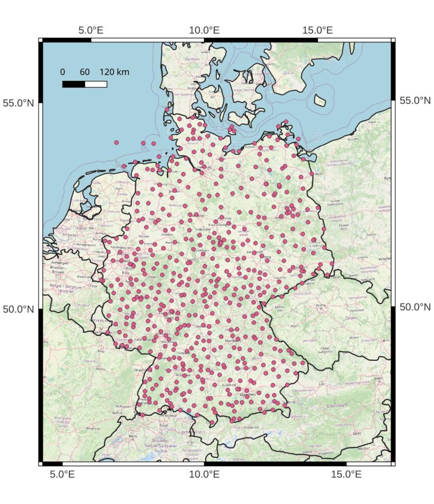
**Figure 1:** Locations of the stations with dew point temperature in Germany. The selection includes only stations with data available from 2001 to 2020 or intervals within this time span.

I downloaded the station data within R (using the rdwd package). The same script also selects only relevant station records and concatenates all station time series in one list that can be easily used later.

Connect tracks with station data and precipitation type

The approach

We want to select a dew point temperature record for each track, preferably from the closest station. Therefore, a record is selected from the closest station at the location of the maximum intensity of a track. To reduce the direct effect of the precipitation event on the dew point measurement, a record between 3 and 4 hours before the event is chosen. The procedure is identical to the one used in Lochbihler et al. (2017). Just in case, I will also extract the dry bulb temperature record from the same station.

Also, each track will be connected with the precipitation type – convective, stratiform and mixed. The data for that comes from an analysis that I covered in a previous post. Since the precipitation type data comes in gridded form each track is associated with a data record from the nearest grid point at the closest time possible.

The final data set

The final data set can be considered more as an add-on. It extends the already existing track database with a number of columns. First, the distance to the closest station (in units of meter) and the corresponding dew point measurement (in degree Celsius). Next, there is the distance to the closest grid point for the precipitation type and then the two criteria, Q1 and Q2.

In R, the final structure of the data set looks like this:

'data.frame':	1920351 obs. of  15 variables:
 $ trID            : chr  "clean-2001-03-21" "clean-2001-03-49" "clean-2001-03-54" "clean-2001-03-87" ...
 $ duration        : num  9 13 6 4 3 5 4 10 6 5 ...
 $ peakvalue       : num  0.23 0.15 0.16 0.13 0.1 ...
 $ peakarea        : int  82 71 50 24 26 22 18 53 30 16 ...
 $ datetime        : POSIXct, format: "2001-03-01 00:15:00" "2001-03-01 00:45:00" "2001-03-01 00:40:00" "2001-03-01 01:00:00" ...
 $ dist            : num  15.18 14 7.67 5.75 7.21 ...
 $ eventtype       : num  1 1 1 1 1 1 1 1 1 1 ...
 $ coorLon         : num  6.65 6.52 14.93 15.09 7.73 ...
 $ coorLat         : num  51.3 53.7 51.3 51.3 47.2 ...
 $ Td_value        : num  -1.7 -0.5 -5.8 -5.7 -9.2 -5.7 -5.7 -7.3 -1.6 -3 ...
 $ Td_distance     : num  8557 41468 9976 16740 76524 ...
 $ CS_grid_distance: num  88046 83894 142236 153386 142884 ...
 $ CS_grid_valueQ1 : num  2 2 2 2 2 2 2 2 2 2 ...
 $ CS_grid_valueQ2 : num  2 2 2 2 2 2 2 2 2 2 ...
 $ TT_value        : num  4.1 1.7 0.2 0.9 -5.7 0.9 0.9 -6.3 2.9 3 ...Code language: JavaScript (javascript)

Code and data

All the code that I used for this analysis is available on github, including basic instructions.

The complete and updated tracks database, can be downloaded from here. With this, you can directly continue with the next part: The analysis.

Part 2: Analysis

Overview and analysis constraints

As mentioned in the previous chapter of this post series, the data quality of the gridded precipitation type data set is time variant. Because of the reduced station data availability after 2015 I will, already at this point, constrain all following analysis to the years from 2001 to 2015.

I will also select only tracks with a maximum duration of two hours. This excludes events which are composed of multiple track life cycles through splitting and merging. The tracking algorithm fails to correctly detect such “freak events”. It is unlikely that this will change the outcomes of the analysis results since less than 7% of events fall into this category.

Station distance and dew point

In the left figure below (Figure 2), we see that the distance of rainfall tracks to the closest station with a dew point record is less than 50km for most tracks. Given the large number of tracks we can, however, make a much stricter selection. I decide to select only tracks with a distance of less than 25km to the closest station, which is still true for about 75% of the data between 2001 and 2015.

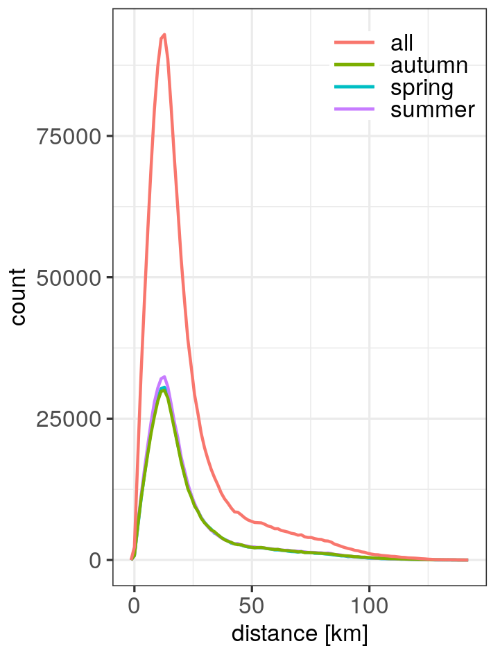
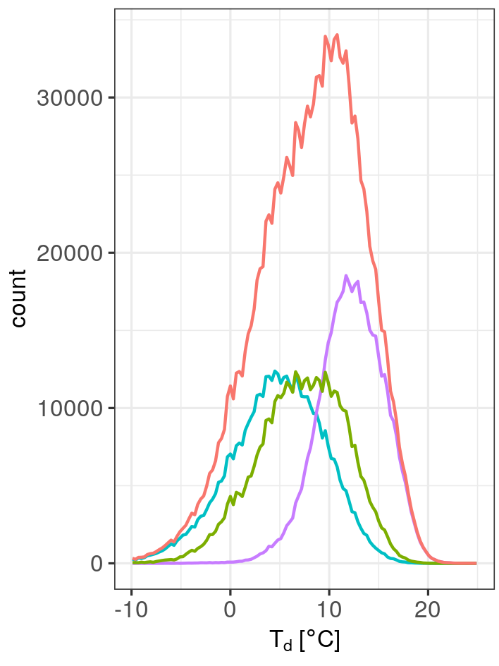
**Figure 2:** Distribution of station distance for assigned dew point temperature records with and without distinguishing seasons.

**Figure 3:** Distributions of assigned dew point temperature (T_d).

There is obviously no substantial difference in the distribution of distances between the seasons. However, when we look at Figure 3, which shows the frequencies of events at a specific dew point temperature, the differences between the seasons become obvious. In spring, events occur generally at lower dew point temperatures followed by events in autumn. Both seasons span a rather wide dew point range with comparable frequencies of evens. In summer, we find a narrower dew point range with higher frequencies. This leads to a skewed distribution if all data is pooled together. The varying dew point ranges in the different seasons is something we should remember for later analysis.

Frequency of precipitation types vs. dew point

Figures 4 and 5 show the event frequency stratified by precipitation type. Both criteria, Q1 and Q2 show a very similar picture. A notable feature is that, in the case of Q2, more events occur with a mixed type as compared to Q1.

The reason is that Q2 is stricter with categorizing a grid cell as convective or stratiform. The consequence is that more events, which are convective or stratiform under Q1, fall into the mixed category in Q2. Figure 6 below shows the difference between the two criteria. Most of the reassignments to the mixed type come from the convective type.

**Figure 4:** Frequencies of rainfall events at specific dew point temperature, grouped by precipitation type criterion Q1. Color coding for seasons is the same as in the Figure above.

**Figure 5:** Frequencies of rainfall events at specific dew point temperature, grouped by precipitation type criterion Q2. Color coding for seasons is the same as in the Figure above/left.

**Figure 6:** The difference in frequencies between Q2 and Q1. Positive values mean that Q2 has higher frequencies at a particular dew point temperature and precipitation type.

We further find that the dew point ranges of the seasons do not vary much between the different precipitation types. However, as noted before (Figure 3), there are considerable shifts in the dew point temperature ranges between the seasons. This leads to a skewed distribution if all seasons are pooled together, at least for the mixed and convective types. The closest resemblance of a normal distribution can be found for the stratiform type.

In summary, based on the results presented so far I will only select tracks for further analysis if they fulfill the following criteria:

no missing values of dew point, Q1 or Q2
the distance to the closest station with a dew point record must be less or equal than 25km
a maximum duration of two hours
between 2001 and 1015

I will also neglect all tracks with a dew point temperature below 0 degree Celsius. In the end, this leaves us with about 0.98 x 10⁶ tracks.

The scaling analysis

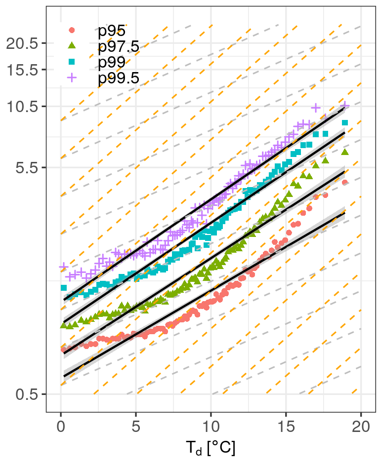
We now know that there is a substantial shift in dew point range from season to season. So, to cover a wider range of dew point temperatures, we have to pool all tracks from all seasons together. Figure 7 shows the resulting scaling diagram for high percentiles of the peak intensity of all events. It becomes clear that these events have a scaling with moisture availability that exceeds the 7% per degree increase of the atmospheres water holding capacity that is given by the Clausius-Clapeyron equation. In numbers, scaling rates range from 9.25%/C^o for the 95th percentile to 10.85%/C^o for the 99.5th.

**Figure 7:** Scaling diagram for extreme rainfall events (high percentiles of peak intensity of events) for all seasons pooled together and without distinguishing between different precipitation types. Each symbol represents a dew point temperature bin with 10,000 members. Grey dashed lines indicate Clausius-Clapeyron scaling (7%/C^o). Orange lines indicate an increase of 14%/C^o. Note the logarithmic y-axis. Intensity is in units mm/5 min.

How does the scaling depend on the precipitation type?

In Figure 8, I grouped events by precipitation type and generated scaling diagrams. I used the stricter Q2 criterion. We can already see visually that scaling rates are substantially higher for convective events than for stratiform events. More specifically, the numbers vary around 11%/C^o vs. 4%/C^o. The mixed type is, as one would expect, settled in between.

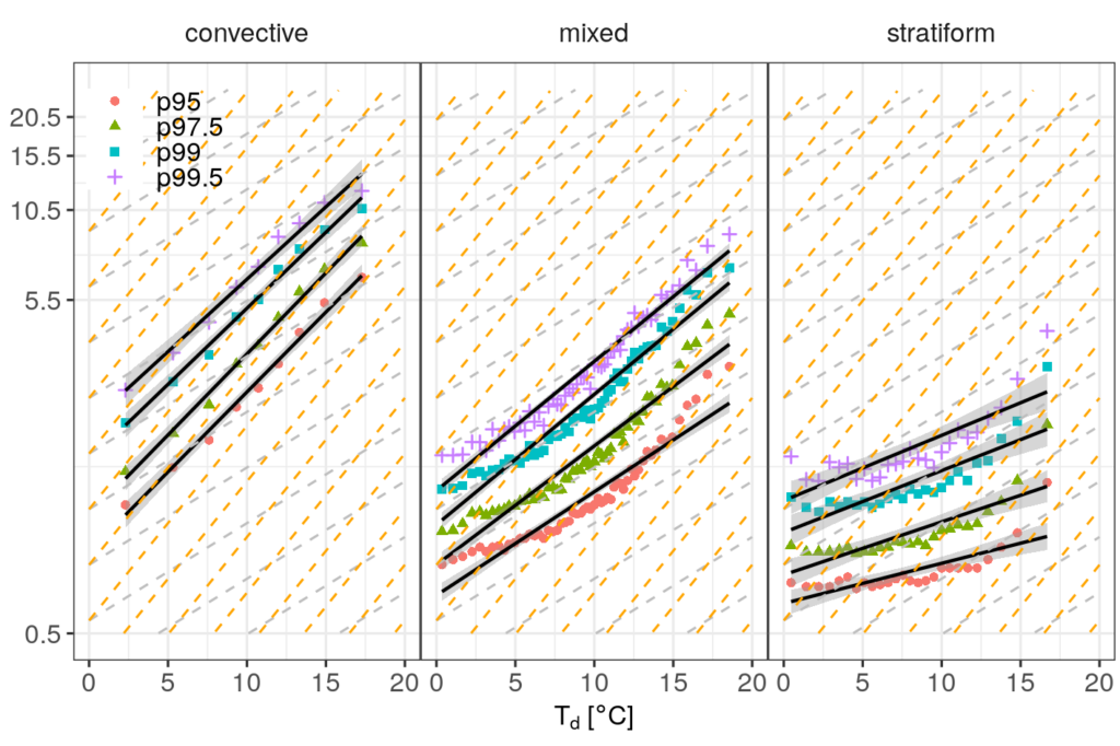
**Figure 8:** Scaling diagrams for different precipitation types (Q2 criterion). Each symbol represents a dew point temperature bin with 10,000 members. Dashed lines indicate Clausius-Clapeyron scaling (7%/C⁰). Orange lines indicate an increase of 14%/C^o. Intensity is in units mm/5 min.

These results are consistent with Moseley et al. (2013), even though the authors used a much more detailed determination of the scaling rate and use the dry bulb temperature as the scaling variable. At some point, I might follow their suggestion and repeat their exact analysis procedure with this new and longer data set.

Summary

For now, I will leave it here. We created a 15 years long precipitation track database where each event is connected to the local moisture availability (dew point) and temperature. Additionally, tracks are associated with one of three precipitation categories – convective, stratiform and mixed.

In line with previous studies, I showed that convective precipitation events exhibit a strong increase of peak intensity with local moisture availability that exceeds the Clausius-Clapeyron rate of 7%/C^o over a wide dew point range. Rainfall tracks that fall into the stratiform category scale at a much lower rate.