In my previous analysis of the event catalog of precipitation events in Germany, I used all available events. And, I already pointed out that the results might be influenced by the type of precipitation event. In this article, I will create a data set that allows us to distinguish between convective and stratiform precipitation events.
This post is part of the germanRADARanalysis project.
The synoptic observations
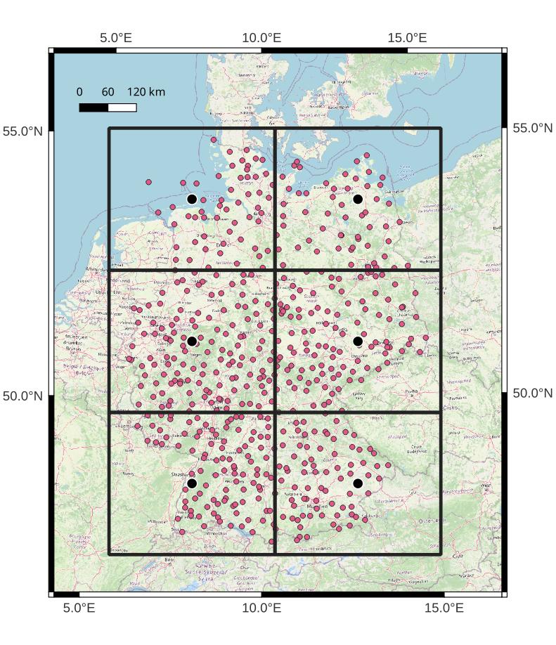
I will use the synoptic observations catalog from the German Meteorological Service (DWD). The zipped archives can be found here. Observations are available on an hourly basis from a total of about 530 stations that have data available for at least a part of the time period from 2001 to 2020. Below you can see a map with all available stations.
Data is available for up to 4 layers of clouds. Here I will use the cloud type in all available layers and the total cloud coverage. The recorded cloud types, the corresponding numeric identifiers and abbreviations are:
| Cloud type | Numeric identifier | Abbreviation |
|---|---|---|
| Cirrus | 0 | CI |
| Cirrocumulus | 1 | CC |
| Cirrostratus | 2 | CS |
| Altocumulus | 3 | AC |
| Altostratus | 4 | AS |
| Nimbostratus | 5 | NS |
| Stratocumulus | 6 | SC |
| Stratus | 7 | ST |
| Cumulus | 8 | CU |
| Cumulonimbus | 9 | CB |
| Instrument | -1 | -1 |
The numeric identifier is -1 for instrumental measurements. In this case, only the height of the cloud layers (not used here) and the cloud coverage is recorded. The latter is measured in fractions of 1/8, and is 0 when no clouds are present. I will also save the cloud coverage.
The grid definition
I generated a grid in QGis with a spacing of 350km in x and 300km in y direction. This leaves us with 2×3 grid cells that cover all available stations in Germany. The map below shows the grid polygons and the corresponding centroids.

The grid cells contain between ~60 and ~130 stations each, depending on their location. For instance, the top-left grid cell contains only 56 stations because it only partly covers Germany. The actual amount of station records can be significantly lower because not all stations have data available at each time step.
The precipitation type definition
This follows the work of Berg and Haerter (2011), Berg et al. (2013) and Moseley et al. (2013).
First, at each time step cloud observations (all cloud layers) at all stations with data records are extracted. Then, for each station it is determined what cloud types are present in the different layers. Each station is labelled “1” if only convective cloud types (8, 9) are present, “2” if only stratiform cloud types (5, 6, 7) are present, and “0” if both types are present.
Then the station labels are collected for each grid box (see figure above) and the precipitation type is determined. I use the two precipitation type descriptors from the sources above.
The first is a rather tolerant distinction between convective and stratiform precipitation:
- A grid cell is considered as the convective type (“1”) if there are no stratiform station labels.
- Conversely, it is labeled as stratiform (“2”) if there are no convective station labels.
- In both cases the presence of mixed cloud types at single stations (class “0”) is allowed, no matter how many there are.
- As soon as there are more than zero of both, convective and stratiform station labels, in a grid box it is marked as mixed precipitation type (“0”).
The second precipitation type descriptor is more strict with point 3. A grid cell can only be considered stratiform or convective if less than half of the station labels are of the mixed type. Otherwise, the grid cell is considered to be a mixed precipitation type, just like in point 4 above.
The first precipitation type descriptor is named Q1, the second Q2.
Variables of the data set
Besides Q1 and Q2, I will also calculate the average total coverage in a grid cell from all available stations with a measurement. Note that the number of stations with a coverage record can be higher than stations with a cloud type record. Not all stations have a cloud type record available at all times and some are using a measuring instrument which does not record the cloud type but the still the coverage.
The number of stations with instrument records is saved in the data set. Furthermore, the total number of stations with a cloud type or instrument record is saved.
The number of stations with missing data records is saved, too. This is done by subtracting the number of stations with a cloud type record or an instrument measurement from the total number of potentially available stations in a grid cell (which is constant over time).
The final data set
Structure
The final data set has 3 dimensions: gridpoint, variable and time steps. The following table explains the details.
| Dimension | Details |
| 1. gridpoint | Index for the six grid points |
| 2. variable | Six variables: Q1, Q2, coverage, nStations, nNA, nInstrument |
| 3. time step | Index for the time steps, hourly. The data set only contains records for the months from March to November. |
Data quality
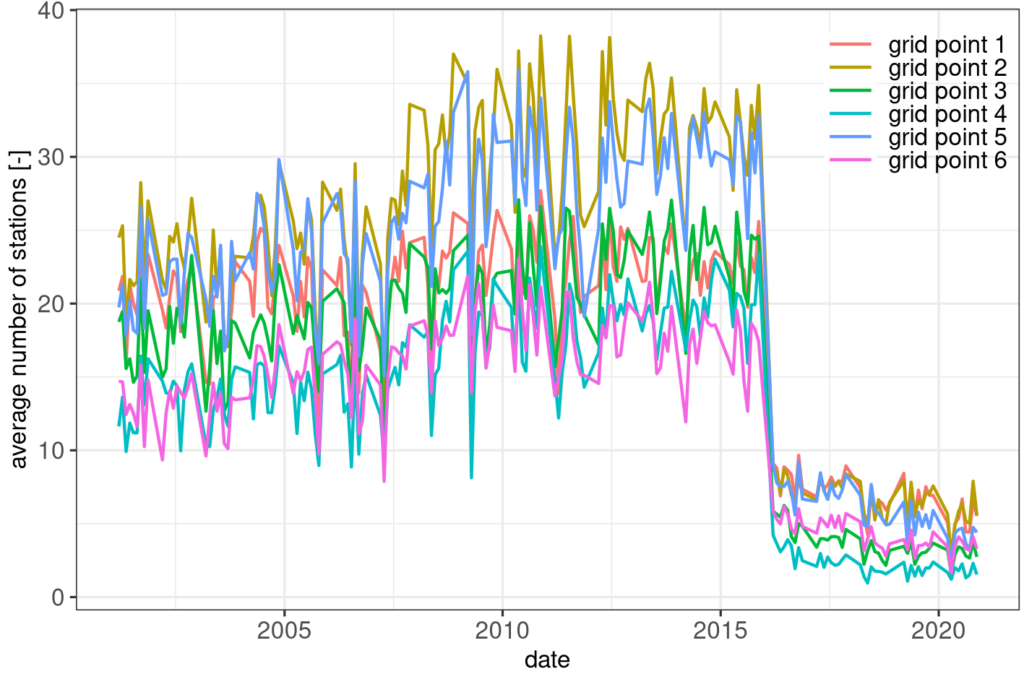
Certainly, a crucial question when generating a gridded data set from station observations is data quality. In this particular case, I want to know how many stations with data are available in each grid cell. The following figure shows how many stations are available for deriving the precipitation type criteria. Because I am interested in changes over time, I calculated monthly averages of data availability.

We can clearly see that the number of available stations is first increasing in all grid cells. Until about the year 2016 when we find a sudden drop.

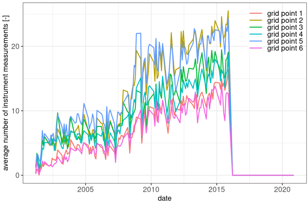
The number of instrument records is also steadily increasing until 2016. Then it drops to zero.
The change in data availability over time poses a challenge for further analysis based on the data set. For now, my suggestion is that the time interval from 2010 to 2015 is safest to use because the number of available stations in this period remains rather constant at a relatively high level.
Download
The data set is available as a zipped RData file and as an archive containing a csv file together with the grid coordinates and a Readme with the description of the variables.
Code
The full R code with all necessary scripts to generate the data set from scratch is available on github.
The script that finally determines the precipitation type for each grid point uses the doFuture package to process the data in parallel. It took about 3 hours on my quad-core CPU and I recommend to have at least 16GB of RAM available.
Further reading
- Description of the synoptic station observations of cloud types in Germany
- The precipitation type definitions for convective, stratiform and mixed classes: Berg and Haerter (2011), Berg et al. (2013) and Moseley et al. (2013).
