High-level scripting languages are great! I mean, you can basically do a complete statistical analysis, including visualizations, with a few lines of code. The thing is that these programming languages, for example R or Python, hide more complex code behind classes, methods and functions. And, very often they call routines that are written in other, lower-level languages, for example C, C++ or even FORTRAN. So what if you want to do something for which there are no existing packages with predefined routines? The answer is simple: do it yourself.
In this exercise, I will show two options of how to implement a specific method in R by using the example of the watershed segmentation. All code and sample data is available on GitHub.
What is watershed segmentation?
First of all, we have to clarify what the watershed segmentation problem is. Wikipedia, of course, has an elaborate article about it and there is a vast amount of literature in the mathematics and computer science world (search ‘watershed transform’). But, for the sake of this article I will keep it very simple with this analogy:
Intuitively, a drop of water falling on a topographic relief flows towards the “nearest” minimum. The “nearest” minimum is that minimum which lies at the end of the path of steepest descent. In terms of topography, this occurs if the point lies in the catchment basin of that minimum.
Wikipedia
The ‘topographic relief’ in this analogy can be anything from a grayscale image to the literal digital elevation model. The name giving example in this sense is the problem of finding the dividing lines between river catchments from topographic data – the watersheds. Here, I will focus solely on the actual catchments, without finding the exact watersheds.
Sample data
To implement and test our algorithm, we need some sample data. As a first, extremely simple data set, we can generate a recurring pattern of pyramids.
pyramids <- matrix(c(0,0,0,0,0,
                     0,1,1,1,0,
                     0,1,2,1,0,
                     0,1,1,1,0,
                     0,0,0,0,0),
                     ncol=5) * -1
pyramids <- cbind(pyramids, pyramids)
pyramids <- rbind(pyramids, pyramids)Code language: R (r)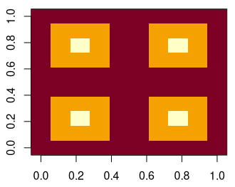
Note that the center of each pyramid is lower in value than the surrounding pixels. Imagine we are looking at the inside of a pyramid. Or, in other words, a funnel.
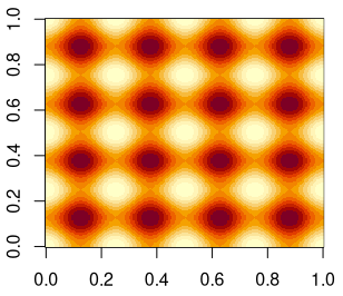
Later, I will also use a more complex example that I created in Gimp. It is a recurring pattern of sine waves in two dimensions.
Description of the algorithm
The algorithm that I use here does the following steps
- Given a matrix of integer or real values, p, with n pixels and dimensions x and y, find all local minima. A pixel p(x,y) is a local minimum if all surrounding pixels have higher values. More specifically, if
- p(x,y) > p(x-1,y) AND
- p(x,y) > p(x-1,y-1) AND
- p(x,y) > p(x,y-1) AND
- p(x,y) > p(x+1,y-1) AND
- p(x,y) > p(x+1,y) AND
- p(x,y) > p(x+1,y+1) AND
- p(x,y) > p(x,y+1) AND
- p(x,y) > p(x-1,y+1)
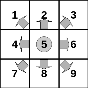
- For each pixel, determine which of the neighboring pixels has the lowest value. This will be used as a direction indicator where a virtual water drop would flow according to the local gradient of the relief. The coding is as follows (see also figure below):
- flow to the upper-left pixel
- flow to the upper pixel
- flow to the upper-right pixel
- flow to the left pixel
- remain at location; local minimum
- flow to the right pixel
- flow to the lower-left pixel
- flow to the lower pixel
- flow to the lower-right pixel
- seed a water drop at each pixel
- move all water drops according to the flow-direction at their current locations
- check if any of the water drops has moved
- repeat steps 4 and 5 until all water drops stop moving
At the end, all drops will have moved to a local minimum. As a sanity check, we can finally check if all drops flowed to a local minimum.
Implementation
Option 1: Code it directly in R
The specific problem in our algorithm is that finding out whether a pixel is a local minimum depends on the neighboring pixels. The same applies to the determination of the gradient at each location. Intuitively, one would solve this challenge by iterating over the dimensions of the matrix and compare the values at each pixel to the neighboring ones. In R, however, this approach comes with a serious performance penalty.
Recently, I stumbled across a smart way to avoid the costly iterations in R with for loops. It was a post on R-bloggers that presents a fast algorithm for Conway’s game of life in R. They achieve a comparison of neighboring cells in a matrix with several shifted copies of the original. So, I thought that this might be an option for my watershed segmentation algorithm in R and I ended up with the following. Object x is the pyramids sample data set from above.
First we create a matrix with each line holding the offset vectors for the shifted copies. The numbers refer to the neighbors in the figure above.
shift.vectors <- matrix(
  c(1, 1,   #1
    1, 0,   #2
    1, -1,  #3
    0, 1,   #4
    0, 0,   #5
    0, -1,  #6
    -1, 1,  #7
    -1, 0,  #8
    -1, -1),#9
    ncol = 2,
    byrow = TRUE
  )Code language: R (r)
Next, we create an array of 9 copies of the original matrix and shift each of them according to the offset values from above. For better readability, I use the ashift function from the magic package.
data.shifted <- array(0.0, dim = c(dim(x)[1], dim(x)[2], 9))
for (i in 1:9) {
  data.shifted[, , i] <- magic::ashift(x, v = shift.vectors[i, ])
}Code language: R (r)
The result is basically a stack of all neighboring pixels. An example: we can select data.shifted[3, 3, ] which will give us all neighbors at positions at x=3 and y=3 in the order from 1 to 9, with 5 being the center pixel. In this case it is the center of the upper left pyramid.
data.shifted[3, 3, ]
[1] -1 -1 -1 -1 -2 -1 -1 -1 -1Code language: R (r)
With a simple call of which.min with apply on the shifted copies we can determine the direction of flow at each pixel.
data.direction <-
    reshape2::melt(apply(data.shifted, FUN = which.min, MARGIN = c(1, 2)))Code language: R (r)
For later purpose, I already reshape the array into a data frame with the explicit coordinate columns. The function (melt) comes from the reshape2 package.
Note, that we actually do not need to explicitly determine the local minima since it is implied in the data.direction matrix. But, we could get the coordinates of all local minima with
data.direction[data.direction[, 3]==5, c(1, 2)]Code language: R (r)Now, we have everything we need to start the flow of water drops along the gradient.
# generate initial coordinates for each drop of the input matrix
init.coor <- expand.grid(seq(1, dim(x)[1]), seq(1, dim(x)[2]))
# initialize, then loop and let drops flow along the gradient
changed <- TRUE
old.coor <- init.coor
new.coor <- init.coor
while (changed) {
  # calculate new coordinates
  new.coor[, 1] <-
    old.coor[, 1] - shift.vectors[data.direction[(old.coor[, 2] - 1) * dim(x)[1] + old.coor[, 1], 3], 1]
  new.coor[, 2] <-
    old.coor[, 2] - shift.vectors[data.direction[(old.coor[, 2] - 1) * dim(x)[1] + old.coor[, 1], 3], 2]
  # boundary checks
  new.coor[new.coor[, 1] > dim(x)[1], 1] <- 1
  new.coor[new.coor[, 2] > dim(x)[2], 2] <- 1
  new.coor[new.coor[, 1] < 1, 1] <- dim(x)[1]
  new.coor[new.coor[, 2] < 1, 2] <- dim(x)[2]
  # check if anything changed
  if (all(new.coor == old.coor)) {
    changed <- FALSE
  } else{
    # update old.coor for next iteration
    old.coor <- new.coor
  }
}Code language: R (r)
Since this approach works with periodic boundaries, we have to check if a drop crossed one or both of the boundaries in each iteration and reset its coordinates to the respective minimum or maximum of the dimensions.
Finally, we label all water drops from their original coordinates, meaning each grid cell of the matrix, with an ID that uniquely identifies the local minimum to which a drop flowed.
data.output <- matrix(0, nrow = dim(x)[1], ncol = dim(x)[2])
loc.min <- as.integer(rownames(data.direction[data.direction[, 3]==5, c(1, 2)]))

for (i in 1:length(loc.min)) {
  data.output[seq(1, dim(x)[1] * dim(x)[2])[(old.coor[, 2] - 1) * dim(x)[1] + old.coor[, 1] ==
					      loc.min[i]]] <- i
}Code language: R (r)
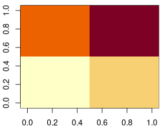
The final result can be visualized with an image plot, here side-by-side with the original.

Or, in raw output…
data.output
      [,1] [,2] [,3] [,4] [,5] [,6] [,7] [,8] [,9] [,10]
 [1,]    1    1    1    1    1    3    3    3    3     3
 [2,]    1    1    1    1    1    3    3    3    3     3
 [3,]    1    1    1    1    1    3    3    3    3     3
 [4,]    1    1    1    1    1    3    3    3    3     3
 [5,]    1    1    1    1    1    3    3    3    3     3
 [6,]    2    2    2    2    2    4    4    4    4     4
 [7,]    2    2    2    2    2    4    4    4    4     4
 [8,]    2    2    2    2    2    4    4    4    4     4
 [9,]    2    2    2    2    2    4    4    4    4     4
[10,]    2    2    2    2    2    4    4    4    4     4Code language: R (r)
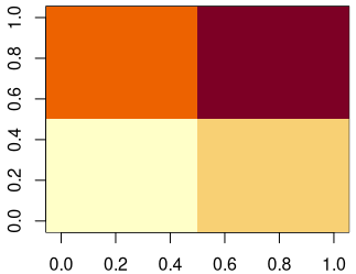
We see that each pixel of the original matrix has an ID that corresponds to its drainage basin (pyramid/funnel).
Option 2: Use a lower-level language as a library
My R implementation tries to exploit the vectorization capabilities of R as much as possible. As a result, it runs much faster than equivalent code with loops. However, if we want to go for maximum speed we should consider outsourcing our algorithm to a library that is written in a compiled language. In my case, I will use FORTRAN, and it happens to be that I already programmed it once for my rain cell tracking tool.
Because the FORTRAN subroutine has more than 250 lines of code, I will spare you the details. But, you can have a look at it here. In a nutshell it does exactly the same as the R implementation but with the option to switch off the periodic boundaries. To use the routine, we first have to compile it,
R CMD SHLIB watershed.f90Code language: Bash (bash)and then load it in R
dyn.load('watershed.so')Code language: JavaScript (javascript)Finally, with the following code we can call the FORTRAN subroutine. x represents the pyramids example data set.
nx <- dim(x)[2]
ny <- dim(x)[1]

retdata <- .Fortran("watershed_simple",
                    # the input matrix x
                    indata = as.double(x),
                    # the output matrix
                    outdata = matrix(rep(as.integer(0), nx * ny), ncol = nx),
		    # dimension size x = dim y in fortran
                    nx = as.integer(ny),
                    # dimension size y = dim x in fortran
                    ny = as.integer(nx),
                    # periodic boundary conditions?
                    periodic = TRUE)Code language: PHP (php)
The final result is identical to the one from the R implementation.
A comparison of performance
Now comes the interesting part. How will the two implementations perform on a larger data set. But first, I want to let you know that I prepared an R package containing all the code and sample data. With this, we can easily run the different implementations and don’t have to worry about the details. Install the package in R with help of devtools by running
require("devtools")
install_github("lochbika/Rwatershed",ref="main")Code language: JavaScript (javascript)
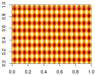
Now, we can run some performance tests. I will use the more complex test data set from the beginning of this post. To make it more interesting, I will replicate the sample data multiple times. At the end we have a 400 x 400 matrix with 2D sine wave patterns.
The results of a simple performance test show that my R implementation takes 30 times longer. So, the compiled FORTRAN code is much faster.
# R implementation
system.time(
+   watershed(sine2d, method = "R", periodic = TRUE)
+ )
   user  system elapsed
  2.086   0.097   2.251

# FORTRAN implementation
> system.time(
+   watershed(sine2d, method = "fortran", periodic = TRUE)
+ )
   user  system elapsed
  0.078   0.000   0.079Code language: PHP (php)
Summary
There are many ways of implementing a method in R. And, I am sure someone can still squeeze out more performance from my R code. But, we have seen that using compiled code as a library in R can significantly speed up things. In the end, it is always a question of how much time someone wants to spend on programming their own functions or whether it is worth at all. If you need a function just a few times and runtime is not critical it is probably not worth to go through the effort of writing C or FORTRAN code to do the job. On the other hand, it is a powerful feature of R to speed up your code significantly. The simple watershed segmentation algorithm that I presented in this post is a good example.